The oil market is hinting at sharp demand destruction

There is a fundamental difference between commodity markets and other markets. The bottom line is: commodity prices must adhere to an underlying physical reality. In contrast, there is no law that demands that equity prices must reflect the operating results and financial prospects of the underlying companies, that currencies have to reflect “fair value” (whatever that is) or that real-estate prices have to be in line with rent, wages or any other driver. Sure, over very long time-horizons, asset prices tend to mean-revert around certain key parameters. But most asset prices can and will divert from these parameters for years, decades in some cases. But in the world of commodities, things stop working quickly when prices become detached from the underlying fundamentals. 

What do we mean by that? First of all, it is important to understand that there is not simply “the price” of a commodity. The most important commodities in the world usually trade on one or several futures exchanges. For example, there is the Brent crude oil contract on the ICE exchange and the West Texas Intermediate (WTI) contract on NYMEX. Both exchanges also have a contract of the respective other grade, although they tend to be less liquid. There are also contracts for dozens of other grades such as Dubai or Western Canadian Select. And many grades that are not trading on future exchanges trade as Swaps. 

Futures contracts are ideally linked to the underlying commodity via the right to delivery[1]. Every exchange has different rules for different contracts. Sometimes the buyer can demand physical delivery, or the seller can force the buyer to take the physical commodity, or sometimes both must agree to physical settlement. Most market participants never get to the point of physical delivery and get rid of their position prior to expiry. 

Hence, for the major commodities in the world, there is a whole host of trades grades and – importantly – tenor. For example, at this very moment point in time, there is a price for the ICE Brent contract closest to delivery. It’s called the prompt. Then there is a price for the next contract, which has delivery one month later and so on. So, for a specific commodity there is a whole set of observable prices over time. This string of prices is called the forward curve (see Exhibit 1). As for every product, there is also a price for the physical good right now at the same point of delivery as the futures contract. It is called the spot price. 

Exhibit 1: The set of observable prices of future contract forms the forward curve

Brent crude oil, $/bbl

Source: GoldMoney Research

Because there are multiple prices for the same commodity (forward curve), similar commodities (grades) and locations (e.g. heavy sour crude in the US gulf coast vs heavy sour crude in the Arab gulf), there are not just many different observable prices but also observable spreads between those prices. As we will show in this report, some of these prices and spreads are more closely linked to the underlying fundamentals than others. 

Flat Price vs spreads

When commodity traders speak about the flat price, they refer to the price of the commodity itself, not a spread. Usually, they mean the prompt contract. One could expect that the flat price of a commodity is directly linked to production costs. Arguably if the price of a commodity falls below the production costs of a producer, one could expect that producers would stop production and the market becomes tighter. However, this mechanism is not as instantaneous as most people think. First, similar to the observation that there is not just one price for a commodity, there is also no “the” production cost of a commodity. There are different levels. For example, the operating costs for an oil project consist of only the costs for labor, material and lease costs for equipment. The all-in costs per barrel of a new offshore oil project includes the costs for exploration, the construction of the oil platform, royalties, interest, maintenance and operating costs as well as the future costs of ecological restoration.

The all-in costs are the most important driver in the decision-making process of a commodity producer whether to go forward with a project or not. An oil company must be convinced that prices over the lifetime of the project will be high enough to cover the all-in costs and allow them to make a profit. 

However, once the project is completed, all-in costs are no longer relevant for whether the company decides to produce. All the money for exploration, building the platform etc. is already spent. Interest has to be paid whether the project produces oil or not. These are all sunk costs. Hence, the decision whether to shut in production when prices drop becomes mostly a function of operating costs. 

Operating costs vary greatly from project to project. Operating costs for large oil projects tend to be just a fraction of total all-in costs. It costs billions of dollars to build an oil platform, but once its built, it needs only a handful of workers and engineers to keep it running for decades. In contrast, operating costs for shale oil production, which is very labor and energy intensive, are closer to 100% of total costs. 

Importantly, once the price of oil drops below operating costs, then the company loses money with every barrel it produces, and it is uneconomical to continue. In some instances, a company might still decide to keep producing at a loss. For example, when labor laws in a specific country make it difficult to lay off people, or when the company is worried it might not be able to rehire people once prices recover. The company might also have sold some of its production forward already, so current prices are irrelevant for some time. Lease agreements might make it difficult for the company to shut in production and restart later. Hence, prices can drop below operating costs and yet producers will still not shut in production for quite some time. Hence operating costs act as a floor to the downside, but the mechanism is far from instantaneous, and prices can be below operating costs for an extended period of time. All-in costs act as an anchor for prices as well as longer-dated future prices need to be high enough to incentivize future production to meet future demand. But that mechanism is even slower and long-dated future prices can be below the marginal cost of future supply for years. 

Commodity prices also can rise substantially above their production costs. The market mechanism to bring balance to the market is that very high production margins incentivize new production and once that production hits the market, prices decline again. But because the lead time of most commodity projects is years, sometimes even more than a decade, this mechanism doesn’t prevent prompt commodity prices from rising substantially over the production costs of future supply. Over the short term, demand is much more responsive to prices than supply. As prices rise higher, consumers of the commodity start substituting. And if that is not possible, they might shut in their manufacturing process altogether as it becomes unprofitable. This has little to do with the production costs of the commodity producer. Hence, there is no reason why commodity prices cannot trade above all-in costs for a prolonged time. 

Therefore, when we say things in the commodity world stop working quickly when prices become detached from the underlying fundamentals, this is only true at the extreme levels when it comes to flat price. Otherwise, the flat price, both prompt and deferred, for most commodities can be detached from underlying fundamentals (costs) for quite some time.

However, that is not true when it comes to spreads. For example, if the price of a commodity in one location is different than the price in another location adjusted for transportation costs, this is usually very short lived. As long as there isn’t a binding reason why a commodity can’t be shipped from one place to another (e.g. due to sanctions), traders will rush in to exploit any arbitrage opportunity. But location spreads are not the only spreads in commodity markets that are bound by underlying fundamentals. The same is true in our view for time-spreads. 

What are time-spreads? Time-spreads are the difference between two contracts of the same commodity with different delivery dates. As we have explained above, the string of all prices of a specific commodity contract is called the forward curve. The forward curve can be flat, upward or downward sloping or a mix thereof. A downward sloping forward curve where the near-dated futures are prices above the longer-dated future is called a backwardated curve. Conversely, an upward sloping curve where the back end is above the front end is called Contango (see Exhibit 2). 

Exhibit 2: Shape of forward curves

Source: Goldmoney Research

So, when is a forward curve in Contango and when in backwardation? One could easily think that each price on the forward curve simply reflects the market’s current expectation of what the price will be at the time of delivery. However, that is incorrect. If this were the case, one could engage in arbitrage. For example, if oil trades at $70/bbl and the 1-year forward contract is at $100/bbl simply because the market thinks the price will be $100 in a year, then a trader could buy the oil now, store it for 12 months (assuming it costs about 50cts/bbl per month to store and insure the crude) and simultaneously sell the 12 month forward at $100/bbl. This would net a profit of $24/bbl. As long as there is this quasi-risk free profit, traders would buy spot and sell the forward (and bid for inventory space). This would lift the prompt price and push the 12-month contract down, until that arbitrage opportunity ceases to exist. Hence, the shape of the curve cannot simply be the market’s expectation for the future price at delivery. 

So, if the slope of a curve is not reflecting the market’s expectation for future prices, what drives the shape? The answer lies in the utility of a commodity at hand for the consumers. When inventories are low, consumers of a commodity have an incentive to pay a premium for immediate delivery. Let’s take the example of an airline. If stocks for jet fuel are very low, the airline must secure supply now, otherwise it faces the risk of running out of jet fuel, which would ground its operations. It’s much more expensive to stop running the business then to pay the premium for jet fuel. Hence, at low inventories, the curve is in backwardation. However, if inventories are very high, then the airline is not at risk of not being able to buy jet fuel when needed. Because storing jet fuel costs money, it would rather make sure it secures fuel for delivery in six months than having it delivered today with the need to store it for six months. But because somebody must store the fuel, that person needs to get compensated to do so. Therefore, the curve must be in Contango, so whoever stores the fuel can buy it cheaper now and sell it more expensively in the future, thus, covering the storage costs. 

From the above, it becomes evident that the shape of the forward curve must be closely related to the level of inventories. And this is where the physical reality in time-spreads comes in. Rising inventories must lead to weaker time-spreads as the holders of more expensive storage must be compensated. There is a merit order for storage in which the cheapest and most easily accessible storage is filled first, and the most expensive last. That means in an environment of rising inventories, the cost for marginal unit of storage is rising.[2] In contrast, when inventories are low and falling, the utility of a barrel delivered today rather than tomorrow is rising. At some point, some consumers need to give up some barrels as there is simply not enough for everybody. Again, there is a merit order where the consumer with the lowest utility are the first consume less. Hence the backwardation of a forward curve increases as inventories decline.

On net, we find that there is an extremely strong correlation between the level of inventories and time-spreads in most commodity markets (see Exhibit 3). We also find that the more a commodity suffers from entropy, the more pronounced this effect is due to storage cost per unit of value. For example, it is extremely expensive to store natural gas in comparison to bauxite. It’s so expensive to store natural gas that inventories typically build close to maximum capacity during injection season of a year and deplete close to tank bottoms during drawing season. For that reason, the natural gas forward curve has a very particular shape with alternating Contango and backwardation over each calendar year. The oil forward on the other hand doesn’t have a seasonal shape, it simply reflects the current level of inventories and to some extent the market’s expectations for inventories in the near future. 

Exhibit 3: There is a very strong correlation between changes in inventories and crude oil time spreads

(LHS) y-o-y change, WTI crude oil 2^nd-3^rd month time spread, (RHS) %, y-o-y change, Cushing stocks, kb

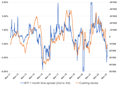
Source: EIA, Goldmoney Research

What does the current shape of the oil forward curve tell us about the state of the economy?

Over the past three years, crude oil time-spreads have been on a rollercoaster. First – as discussed above – they completely collapsed on the back of the lockdown induced demand destruction. Then, they recovered as inventories gradually declined due to OPEC+ unprecedented supply cuts. By late 2021, demand was close to pre-COVID levels. After that the war in Ukraine started and with it came the fear that we would run out of oil globally as more and more Russian oil production appeared to be a risk, be it either from sanctions or possibly due to Russia’s trying to destabilizing the oil market. Global inventories dropped to dangerously low levels, but more importantly, the market priced in high probability of forward supply losses which implied even lower forward inventories. Crude oil time-spreads went from all-time lows in 2020 to all-time highs in early 2022. But as those fears about Russian supply losses and thus further inventory draws didn’t materialize, time-spreads retreated and we entered a period of more “normal” backwardation, in line with the low but manageable global petroleum stocks. 

However, over the past few months, we have seen a collapse in time-spreads. While this coincided with an increase in inventories in the US, our models suggest that time-spreads are now much weaker than the underlying stocks imply. The surprise OPEC+ announcement of a production cut of over 1.5mb/d on April 2, 2023 has led to some recovery in time-spreads, but even now time-spreads are weaker than current inventories imply.

This means that prior to the cut, the oil market was pricing in that crude oil inventories will rise substantially over the coming months. More specifically, the Brent time-spreads implied a 100mb or 1.75mb/d build over the next 8 weeks. WTI time-spreads were already in Contango, implying a 200mb or 3mb/d build (see Exhibit 4). This would require a large crude oil oversupply. Importantly, this is based on US inventories alone. Because it is unlikely that US stocks would build that much while inventories in the rest of the world remain flat, the global crude overhang would have to be even larger.

Exhibit 4: WTI time-spreads imply a large building US total petroleum stocks going forward

$/bbl

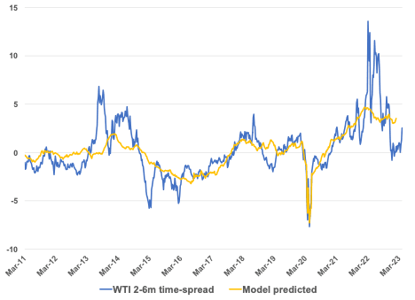
Source: Goldmoney Research

As the supply situation is not expected to change dramatically going forward, the only way we could see such a large crude overhang materializing is by a sharp decline in demand on the back of a major recession. How steep of a recession does this imply? To put things into perspective, crude oil demand is roughly growing at around the rate of global GDP -2%. The 2% is due to efficiency gains.[3] 

A healthy real global GDP growth is somewhere around 3-4% (real meaning nominal growth – inflation). That typically translates into oil demand growth at around 1-2mb/d. According to the International Monetary Fund (IMF) real global GDP grew 3.4% last year after going through a rollercoaster ride in 2020 and 2021. In 2022, oil markets were roughly balanced, meaning commercial inventories moved more or less with the seasonal average, albeit at a very low level. However, part of the reason was that the US government released a record 600kb/d of crude oil on average throughout the year (see Exhibit 5). This means that in 2022, global production was lagging global demand by 600kb/d and the only reason we didn’t see commercial inventories drawing was because the US government stocks drew instead. Hence, without the release of 600kb/d of crude from the US SPR, the market would have been in deficit.

Exhibit 5: The US government released a record 600kb/d of crude from the SPR in 2022

(LHS) kb/d, (RHS) level kb

Source: Goldmoney Research

For 2023, the IMF sees a slowdown in global growth, but only to 2.9%. Without the US SPR barrels – all else equal – this would bring the market back to balance. 

This is in line with US crude oil inventories. While January and February saw larger than normal builds, March had a large draw again (see Exhibit 6). 

Exhibit 6: US crude oil stocks were weaker than normal in the first two months of the year, but March was stronger than normal

Kb/d

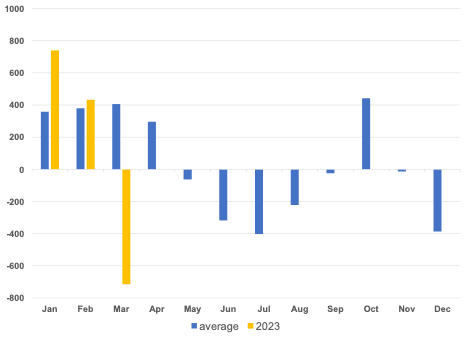
Source: EIA, Goldmoney Research

Total petroleum stocks – including products such as gasoline and diesel – looked very weak in January and February. But March saw a much larger than normal draw. Overall total petroleum stocks were weaker than normal in 1Q23, but only by about 200kb/d (see Exhibit 7)

Exhibit 7: US total petroleum stocks built much faster in the Jan-Feb 2023 period than they seasonally do, but a lot of that reversed in March 2023

Kb/d

Source: EIA, Goldmoney Research

Crude oil time-spreads have weakened not just when the inventory picture looked weaker than normal, but also in March, when inventories saw large draws in the US and even as OPEC announced the cut. 

Thus, the crude oil market seems to be pricing in substantial demand destruction going forward. An oversupply of 2-3mb/d would imply a hit to GDP of 2-3%. This would imply a global recession, similar in magnitude than the 2008 GFC. If this were to materialize however, it would unlikely be limited to 2Q23. It is also interesting to see that the surprise oil cut by OPEC couldn’t bring time-spreads fully back in line with inventories. This is further evidence that the market was pricing in more than a 1.5mb/d demand destruction. -1.5% demand equates to around 1.5% lower GDP growth. 

On net, the oil market has shifted from signalling extremely tight forward inventories to quite loose forward inventories in a very short amount of time. In our view, this could only materialize if we are entering a global recession. The ingredients for such a scenario are certainly there. However, we haven’t seen these large surpluses materialize just yet. If a global recession were to materialize, OPECs surprise cut would only help to balance the oil market short term. It may also speed up and / or exacerbate the recession for two reasons. First, in an economic slowdown, companies and consumers at least get some relief from lower commodity prices. OPEC’s moves offset this effect at least short term. Second, and more importantly in our view, it keeps inflationary pressure higher and may force central banks to raise rates higher and keep them there for longer than they would otherwise do. 

If we do see a recession of similar magnitude than in 2008, the current OPEC cut will not be enough.  Back then, oil demand declined globally by 4%. With current global demand, that would be around 4 million b/d. However, OPEC+ is in a very different position now than it was in 2008. The resounding success of the unprecedented 2020 cuts due to the COVID19 lockdowns have shown that OPEC has the means and the will to balance markets if necessary. It would be quite challenging for central banks to react to a sharp economic slowdown yet stubbornly high inflation. 

[1] There are futures contracts for commodities without a delivery mechanism. Usually those are purely financially settled and the final price at expiry is based on an assessment. For example, the JKM LNG contracts are based on a medley of reported landed prices in various locations. This means there is no mechanism that pushes the futures price towards the physical price as there is no effective arbitrage. 

[2] It can be that at some point, all storage space is used up. At that point, it is the flat price that will reach a level where producers have no other choice than to shut in. This happened in the most impressive way in spring 2020. The first global lockdown during the COVID19 pandemic lead to an unprecedented demand destruction for petroleum products. Inventories in the US built at record speed, but at some point, the market became seriously concerned about storage containment issues, particularly at the Cushing Oklahoma hub. The Cushing hub is the point of delivery for the WTI crude oil contract. This was exacerbated by the fact that some non-commodity players held substantial long positions all the way until two days before expiry of the April contract. These were funds – particularly one – that offered crude oil exposure to their clients by being long the prompt contract and rolling it into the successive contract when the prompt was about to expire. While the liquidity in crude oil futures is very high and this strategy might not cause much of an issue in normal times, when the April 2020 contract came close to expiry, there was nobody to offload these contracts to. The reason was that nobody had enough empty storage at Cushing to receive these barrels. As a result, prices dropped as low as $-40/bbl. This was then enough to have some market participants that still had some wiggle room to act (for example somebody could have paid a producer to not produce barrels that were already sold and scheduled for delivery). 

[3] Historically, efficiency gains came mainly on the back of better fuel economy of ICE vehicles. Over recent years, we have seen a shift though. While it becomes increasingly difficult to achieve further efficiency gains in ICE vehicles, the rise of EV (both full EVs and Hybrid vehicles) means that global fuel consumption continues to lag global GDP. Now, the share of EVs sold is too small to alter the efficiency gain beyond the historical rate, but eventually we expect that to happen.